最后更新: 2025-02-17 15:54 查看: 154 次纠错评论(0) 课件开VIP

附录：利用机器学习预测房价

房价预测是机器学习中基本的知识点，也是理想的了解机器学习原理的知识点。获取数据：数据集下载见以下链接：
链接：https://pan.baidu.com/s/1qPXdvb0oskZjv4cGw3hPrQ
提取码：qvk1

## 1.基本数据样子
一个城市的房价收到：房屋的年限，面积，层数，房间数，浴室，价格六大因素的影响（这里仅仅用这六个参数作为距离，实际影响参数远远不止六个）。

![图片](/uploads/2025-02/40355a.jpg)
 
    2.单因素分布
 　这不是一个很大的数据，也没有太多的列，因此第一步可以绘制直方图，查看下各因素的数据分布情况。
  
  ```
  import pandas as pd
import matplotlib.pyplot as plt
df1 = pd.read_csv(r"./house_data.csv")
#直方图
df1.hist(bins=20,figsize=(10,10))
plt.show()

```
  效果：
  
   ![图片](/uploads/2025-02/058f39.jpg)
   
   
 ## 特征，线性回归
 这些影响房价的因素，我们又称之为“特征”。这些特征是如何影响房价的？就好比x,y，我们来看下各特征与房价间的关系图
 ``` 
import pandas as pd
import seaborn as sns
import matplotlib.pyplot as plt
house = pd.read_csv(r"./house_data.csv")
house = house.astype(float)
col1 = house.columns
# 生成图表
for col in col1:
    f, ax = plt.subplots(1, 1, figsize=(12, 8), sharex=True)
    sns.regplot(x=col, y='price', data=house, ax=ax)
    x = ax.get_xlabel()
    y = ax.get_ylabel()
    ax.set_xlabel(x, fontsize=18)
    ax.set_ylabel(y, fontsize=18)
    plt.show()
```

![图片](/uploads/2025-02/df857d.jpg)
 
 ## 特征，箱型图

为了确定卧室数量、卫生间数量、楼层数与价格的比较，OF更喜欢箱型图，因为有数字呈现，但它们不是连续的，如 1,2,... 卧室，2.5, 3,... 楼层（可能 0.5 代表阁楼 ）。

结论：

通过箱型图，去除一些黑点的异常值，我们可以发现，曲线上升比较明显的有房屋面积、卫生间数量，还有卧室数量也有些微小的曲线上升，那么我们可以认为整体上，房价与这3个特征有关系。
  ```
  import pandas as pd
import seaborn as sns
import matplotlib.pyplot as plt
house = pd.read_csv(r"./house_data.csv")
house = house.astype(float)
col1 = house.columns
# 生成图表
for col in col1:
    f, ax = plt.subplots(1, 1, figsize=(12, 8), sharex=True)
    sns.boxplot(x=house[col],y='price', data=house, ax=ax)
    x = ax.get_xlabel()
    y = ax.get_ylabel()
    ax.set_xlabel(x, fontsize=24)
    ax.set_ylabel(y, fontsize=24)

plt.show()

```

![图片](/uploads/2025-02/e061a0.jpg)
 
 ## 变量相关性

模型中有太多特征并不总是一件好事，因为当我们想要预测新数据集的值时，它可能会导致过度拟合和更糟糕的结果。如果想要一眼看出各变量间的关系，不得不向大家介绍皮尔逊相关性矩阵，用热图来呈现。
   ![图片](/uploads/2025-02/9137eb.jpg)
   
   　怎么看这张图？很简单，右侧的颜色色条中向上红色加深代表正相关；向下蓝绿色加深代表负相关（绝对值越大，相关性越大）。因为我们主要分析各变量与房价间的关系，所以我们比较最下一行的数据。

square房屋面积 0.7 > bathrooms卫生间数量 0.53 > bedrooms 0.31 > floos 0.26
  
  ## 多因素，3D

上述绘制了房价与其他因子的对比，似乎价格与这些因子之间没有完美的线性关系。3个变量彼此之间的关系又如何？
  ``` 
import numpy as np
import pandas as pd
import seaborn as sns
import matplotlib.pyplot as plt
import itertools
from mpl_toolkits.mplot3d import Axes3D
plt.rcParams['font.sans-serif']=['SimHei'] #显示中文标签
plt.rcParams['axes.unicode_minus']=False   #这两行需要手动设置
house = pd.read_csv(r"./house_data.csv")
house = house.astype(float)
hs2 = house.drop(['price'],axis=1)
col1 = house.columns
col2 = hs2.columns
combine = pd.DataFrame(itertools.combinations(col2, 2))
for i in range(len(combine)):
    fig = plt.figure(figsize=(10,6))
    ax = Axes3D(fig)
    x=house[combine[0][i]]
    y=house[combine[1][i]]
    z=house['price']
    ax.scatter(x,y,z)
    plt.title("三维分析"+combine[0][i]+"-"+combine[1][i]+"-"+"price",fontsize=18)
    ax.set_xlabel(combine[0][i],fontsize=14)
    ax.set_ylabel(combine[1][i],fontsize=14)
    ax.set_zlabel('price',fontsize=14)
    plt.tick_params(labelsize=10)
    plt.show()
```

![图片](/uploads/2025-02/27862a.jpg)
 
 经过线性回归、箱型图、皮尔逊相关性矩阵和3D图的分析，都能分析出来房价与房屋面积、卫生间数量有比较大的关系。下期将会涉及一些机器学习的知识来预测房价
 
 ## 预测
1.说明

主要是房屋面积、卫生间数、卧室数。今天，我们通过建立模型来预测房价。机器学习中关于回归算法-数据发展的预测，包含了几个模型

1、线性回归；

2、岭回归；

3、Lasso回归；

4、多项式回归。

2.线性回归

线性回归的公式很简单y=ax+b（a是系数，b是截距），借这个简单的公式来介绍下机器学习的过程。
   ![图片](/uploads/2025-02/5dcc2d.jpg)
   
   步骤：

1、定义训练集、测试集；

2、选择模型；

3、训练模型；

4、预测和推断。

``` 
import numpy as np
import pandas as pd
from sklearn.model_selection import train_test_split
from sklearn import linear_model
import matplotlib.pyplot as plt
import tkinter as tk

df = pd.read_csv(r"./house_data.csv")
#定义训练集、测试集
train_data,test_data = train_test_split(df,train_size = 0.8, random_state=3)
#定义训练数据列
X_train = np.array(train_data['square'], dtype=pd.Series).reshape(-1,1)
y_train = np.array(train_data['price'], dtype=pd.Series)

#定义测试数据列
X_test = np.array(test_data['square'], dtype=pd.Series).reshape(-1,1)
y_test = np.array(test_data['price'], dtype=pd.Series)

#选择模型
lr = linear_model.LinearRegression()

# 训练模型
lr.fit(X_train,y_train)

#预测、推断
pred = lr.predict(X_test)
```

看看效果：

将预测值，与target进行对比，画图

#图表显示
plt.scatter(X_test, y_test)
plt.plot(X_test,pred,color='r')
plt.show()

我们来看下的线性回归是一条怎样的线（下图红色线）：
  
   ![图片](/uploads/2025-02/bca2e4.jpg)
   
   
   　模型评价：

从肉眼上看，这条线性回归效果似乎并不太理想，我们用数据说话，计算下该模型的评分如何。我们一般用以下指标来衡量模型的好坏：R2（决定系数）、RMSE（均方根误差）、cv（K折交叉验证系数）。

#计算模型评分
X = np.array(df['square']).reshape(-1,1)
print(lr.score(X,df['price']))
 　
  得分：

D:\Python310\python.exe E:/bme-job/torchProjectDemo/houseprice/linear.py
0.4928363894587906

Process finished with exit code 0

### 线性预测：

R2分数越高，说明模型的准确率越高，低于50%的准确率，模型确实不太理想啊。但既然做出来了，我们用该模型预测下房价。
  
  ``` 
###
# 计算系数和截距
coef = float(lr.coef_)
intercept = float(lr.intercept_)
print('系数 Coefficient: {}'.format(coef))
print('截距 Intercept: {}'.format(intercept))

print("Average Price for Test Data: {:.3f}".format(y_test.mean()))

# 第1步，实例化object，建立窗口window
window = tk.Tk()
# 第2步，给窗口的可视化起名字
window.title('房价预测计算器-线性回归')
# 第3步，设定窗口的大小(长 * 宽)
window.geometry('500x300')  # 这里的乘是小x
# 第4步，在图形界面上设定输入框控件entry框并放置
a = tk.Label(window, text="房屋面积：")
a.place(x='30', y='50', width='80', height='40')
e = tk.Entry(window, show=None)  # 显示成明文形式
e.place(x='120', y='50', width='180', height='40')

# 第5步，定义触发事件
def calculate():  # 在鼠标焦点处插入输入内容
    var = e.get()
    ans = coef * float(var) + intercept
    ans = '%.2f' % ans
    result.set(str(ans))

# 第6步，创建并放置一个按钮
b1 = tk.Button(window, text='预测房价', width=10, height=2, command=calculate)
b1.place(x='320', y='50', width='100', height='40')
# 第7步，创建并放置一个多行文本框text用以显示
w = tk.Label(window, text="预测房价（万元）：")
w.place(x='50', y='150', width='120', height='50')
result = tk.StringVar()
show_dresult = tk.Label(window, bg='white', fg='black', font=('Arail', '16'), bd='0', textvariable=result, anchor='e')
show_dresult.place(x='200', y='150', width='250', height='50')
# 第8步，主窗口循环显示
window.mainloop()
```

效果：

D:\Python310\python.exe E:/bme-job/torchProjectDemo/houseprice/linear.py
0.4928363894587906
系数 Coefficient: 1.94438675017008
截距 Intercept: -30.230797817428652
Average Price for Test Data: 345.436
　　图：
   ![图片](/uploads/2025-02/83b2ab.jpg)
   
   总结：

y = 1.94438675017008 * x + (-30.230797817428652)

### 3.岭回归

线性回归呈现了房价与房屋面积的关系，但实际上，房价的影响因素可不止面积，还有卫生间数量和卧室数量，当然还有其他一些特征。我们本次用这3个特征进行岭回归预测。岭回归的公式：
  
  ``` 
import pandas as pd
from sklearn.model_selection import train_test_split
from sklearn import linear_model
import tkinter as tk

"""
岭回归
"""

# 训练集与测试集
df_dm = pd.read_csv(r"./house_data.csv")
train_data_dm, test_data_dm = train_test_split(df_dm, train_size=0.8, random_state=3)

# 训练
features = ['square', 'bathrooms', 'bedrooms']
complex_model_R = linear_model.Ridge(alpha=100)
complex_model_R.fit(train_data_dm[features], train_data_dm['price'])

# 预测
pred1 = complex_model_R.predict(test_data_dm[features])
intercept = float(complex_model_R.intercept_)
coef = list(complex_model_R.coef_)
print('系数 Coefficients: {}'.format(coef))
print('截距 Intercept: {}'.format(intercept))

# 计算模型评分
print(complex_model_R.score(df_dm[features], df_dm['price']))

# 使用图形进行展示
# 第1步，实例化object，建立窗口window
window = tk.Tk()
# 第2步，给窗口的可视化起名字
window.title('房价预测计算器-岭回归')
# 第3步，设定窗口的大小(长 * 宽)
window.geometry('500x350')  # 这里的乘是小x
# 第4步，在图形界面上设定输入框控件entry框并放置
a = tk.Label(window, text="房屋面积：")
a.place(x='30', y='50', width='80', height='40')
e = tk.Entry(window, show=None)  # 显示成明文形式
e.place(x='120', y='50', width='180', height='40')
b = tk.Label(window, text="卫生间数：")
b.place(x='30', y='120', width='80', height='40')
f = tk.Entry(window, show=None)  # 显示成明文形式
f.place(x='120', y='120', width='180', height='40')
c = tk.Label(window, text="卧室数：")
c.place(x='30', y='190', width='80', height='40')
g = tk.Entry(window, show=None)  # 显示成明文形式
g.place(x='120', y='190', width='180', height='40')

# 第5步，定义触发事件
def calculate():  # 在鼠标焦点处插入输入内容
    var1 = e.get()
    var2 = f.get()
    var3 = g.get()
    ans = coef[0] * float(var1) + coef[1] * float(var2) + coef[2] * float(var3) + intercept
    ans = '%.2f' % ans
    result.set(str(ans))

# 第6步，创建并放置一个按钮
b1 = tk.Button(window, text='预测房价', width=10, height=2, command=calculate)
b1.place(x='350', y='120', width='100', height='40')
# 第7步，创建并放置一个多行文本框text用以显示
w = tk.Label(window, text="预测房价（万元）：")
w.place(x='30', y='250', width='120', height='50')
result = tk.StringVar()
show_dresult = tk.Label(window, bg='white', fg='black', font=('Arail', '16'), bd='0', textvariable=result, anchor='e')
show_dresult.place(x='200', y='250', width='250', height='50')
# 第8步，主窗口循环显示
window.mainloop()
```

效果：

D:\Python310\python.exe E:/bme-job/torchProjectDemo/houseprice/ridgeregression.py
系数 Coefficients: [2.1476306373305176, 3.273168924436608, -35.96335039929463]
截距 Intercept: 44.842680015586325
0.5068817650838495

Process finished with exit code 0

该模型计算得到的评分稍微要高一些：

上面可以看到是0.5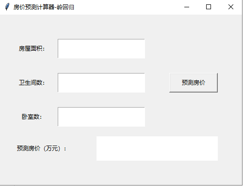
   ![图片](/uploads/2025-02/576ed9.jpg)
   总结：

h = coef[0] * float(var1) + coef[1] * float(var2) + coef[2] * float(var3) + intercept

4.Lasso回归

1）Lasso回归的公式：
2）岭回归与Lasso回归的公式是相同的，Lasso回归与岭回归的区别在于：

Many small/medium sized effects: 使用（Ridge）岭回归

Only a few variables with medium/large effect: 使用Lasso回归

3）岭回归也称为L2 正则化，Lasso回归也称为L1正则化

岭回归与Lasso回归最大的区别在于岭回归引入的是L2范数惩罚项，Lasso回归引入的是L1范数惩罚项，Lasso回归能够使得损失函数中的许多θ均变成0，这点要优于岭回归，因为岭回归是要所有的θ均存在的，这样计算量Lasso回归将远远小于岭回归。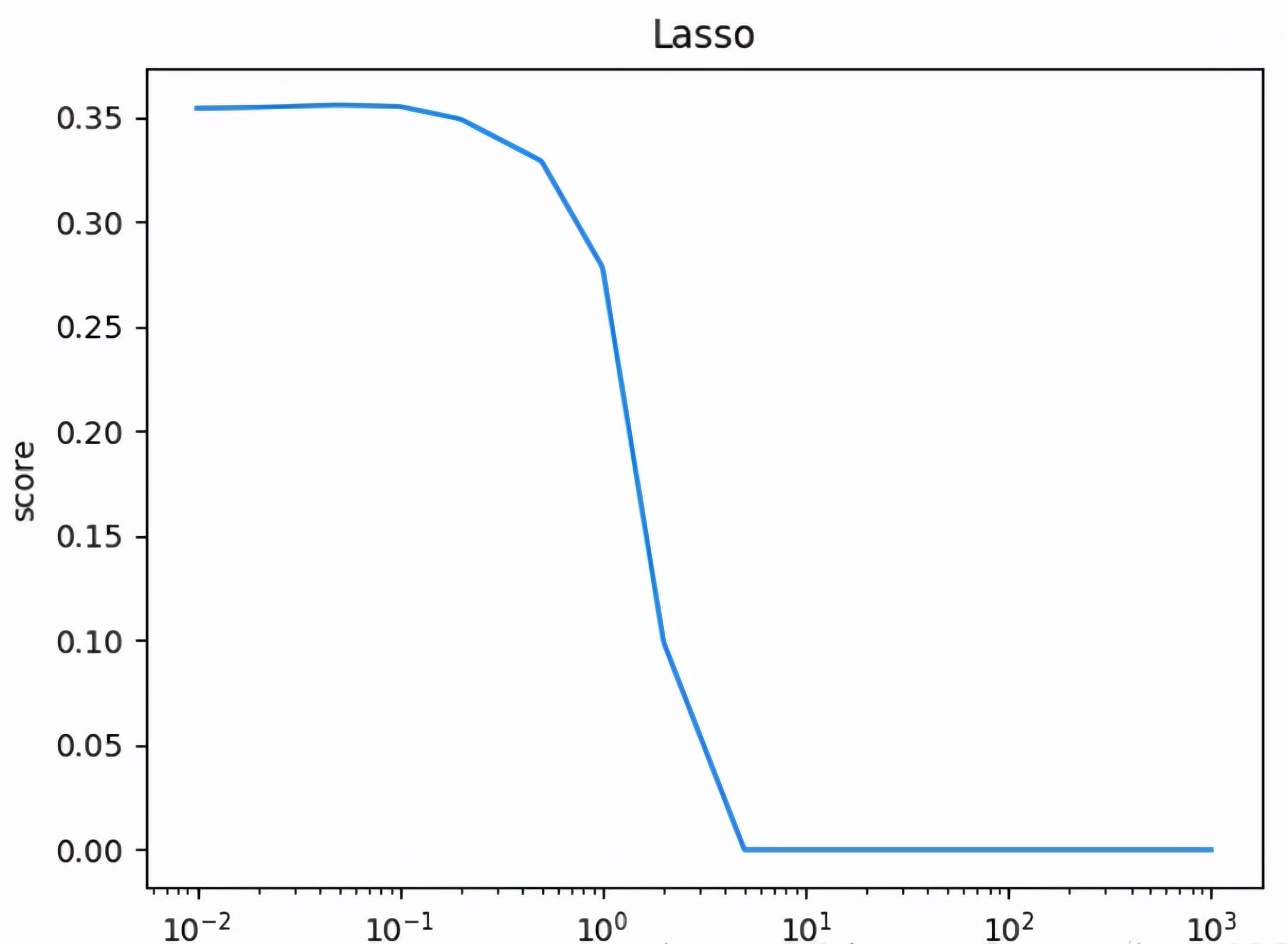
   ![图片](/uploads/2025-02/3fb691.jpg)
   
   ``` 
   import pandas as pd
from sklearn.model_selection import train_test_split
from sklearn import linear_model
import tkinter as tk

"""
岭回归
"""

# 训练集与测试集
df_dm = pd.read_csv(r"./house_data.csv")
train_data_dm, test_data_dm = train_test_split(df_dm, train_size=0.8, random_state=3)

# 训练
features = ['square', 'bathrooms', 'bedrooms']
complex_model_R = linear_model.Lasso(alpha=100)
complex_model_R.fit(train_data_dm[features], train_data_dm['price'])

# 计算模型评分
print(complex_model_R.score(df_dm[features], df_dm['price']))

```

效果：

D:\Python310\python.exe E:/bme-job/torchProjectDemo/houseprice/Lassoregression.py
系数 Coefficients: [1.9306318375107603, -0.0, -0.0]
截距 Intercept: -27.571319416416088
0.4928520192488185

Process finished with exit code 0

### 5.多项式回归

多项式回归的公式：略
  
  
  参考
  https://blog.csdn.net/weixin_42341655/article/details/120299008?spm=1001.2014.3001.5501

https://blog.csdn.net/weixin_42341655/article/details/120340827

科数题库(单机版) 会议室预约系统(book)

今日还可看 0 篇未注册用户每天查看4篇，注册用户每天8篇，开通VIP会员无限制查看。

免费注册

《高等数学》难点解析

高数教程 泰勒公式切线与法线切平面与法平面驻点·拐点·极值点·零点间断点渐进线瑕积分欧拉方程伯努利方程 Abel 收敛定理偏导数的几何意义偏导数的几何意义梯度数量场与向量场多元函数极值拉格朗日算子通量与散度环流量与旋度格林公式高斯公式斯托克斯公式三大公式比较傅里叶级数极坐标微元点法式方程变上限定积分 X型计算面积 Y型计算面积微分的意义渐近线间断点 y''+py'+qy=f(x)方程高斯黎曼傅里叶变换(复数) 拉普拉斯变换(复数)

《线性代数》难点解析

线代教程 近世代数对数学的整体思考线性的意义矩阵乘法(列视角) 矩阵乘法(行视角) 矩阵左乘矩阵右乘逆矩阵求解方程组阶梯形矩阵的求法方程组解的判定四阶行列式的计算线性变换的意义线性空间向量组的等价线性空间的几何意义基础解系的求法施密特正交化特征值与特征向量的意义矩阵相似的几何意义矩阵可对角化的理解秩的意义(向量版) 秩的意义(方程版) 二次型的意义

《概率论与数理统计》难点解析

概率教程 置信区间与上a分位数概率中的“取”与“放” 贝叶斯公式全概率公式泊松分布指数分布伽玛分布二维密度图的意义卷积的意义相关系数的意义 k阶矩是与矩母函数卡方分布的作用单正态区间估计理解假设检验理解切比雪夫不等式中心极限定理

上一篇：旧版本

下一篇：没有了

本文对您是否有用？有用 (0) 无用 (0)